Generalized Linear Models

Motivation

We can address a larger amount of problems and models by abstracting a general for of linear models to account for categorical responses types such as binomial, multinomial, and poisson.

A GLM is defined by specifying two components:

response: member of the exponential family distribution
link function: describes how the mean of the response and a linear combination of the predictors are related

Components

The distribution of \(Y\) is from the exponential family of distributions, and takes the general form of:

\[f(y|\theta, \phi) = exp(\frac{y\theta - b(\theta)}{a(\theta)} + c(y, \theta))\]

\(\theta\): canonical parameter, represents the location
\(\Theta\): dispersion parameter, represents the scale
\(a, b, c\): define various members of the family by specifying these

Common GLMs

Binomial Distribution
Poisson Distribution

GLM Setup

Let

\(x_j = (x_{1, j}, \dots x_{n, j})^T\), \(j=1, \dots, p\) be a set of predictors
\(Y = (Y_{1}, \dots Y_{n})^T\)
\(\beta = (\beta_0, \beta_1, \dots, \beta_p)^T\)

A GLM has three components:

Random Component:
- refers to the probability distribution of the response variable (i.e. binomial distribution)
- a random variable from the exponential family if the distribution can be written as the exponential function above
Systematic Component:
- refers to the explanatory variables \((X_1, \dots, X_k)\) as a combination of linear predictors
- \(\eta = \beta_0 + \beta_1 x_1 + \dots \beta_p x_p = x^T\beta\)
Link Function:
- specifies the link between the random and systematic components
- describes how the expected value of the response relates to the linear predictor of explanatory variables
- link function, \(g\), describes how the mean response, \(E[Y] = \mu\) is linked to the covariates through the linear predictor: \(\eta = g(\mu)\)
- i.e. \(\eta = logit(\pi)\) as in logistic regression
- we require a monotone continuous and differentiable function

Log-Likelihood

log-likelihood function: \(l(\theta) = \frac{y\theta - b(\theta)}{a(\phi) + c(y, \phi)}\)
derivative wrt \(\theta\): \(l'(\theta) = \frac{y - b'(\theta)}{a(\phi)}\)
expectation over \(y\): \(E[l'(\theta)] = \frac{E[y] - b'(\theta)}{a(\phi)}\)

From general likelihood theory, we know that \(E[l'(\theta)] = 0 \rightarrow E[Y] = \mu = b'(\theta)\)

second derivative: \(l''(\theta) = -E[(l'(\theta))^2]\)
\(\frac{b''(\theta)}{a(\phi)} = \frac{E[(Y - b'(\theta))^2]}{a^2(\phi)}\)
results in: \(var(Y) = b''(\theta)a(\phi)\)

Binomial Regression (Logistic Regression)

\(f(y|\theta, \phi) = \binom{n}{y} \mu^y (1-\mu)^{n-y}\)

\(= exp(ylog\mu + (n-y)log(1-\mu) + log\binom{n}{y})\)

\(= exp(ylog\frac{\mu}{1-\mu} +nlog(1-\mu) + log\binom{n}{y})\)

\(\theta\) (canonical parameter): \(log\frac{\mu}{1-\mu}\)
\(b(\theta)\): \(-nlog(1-\mu) = nlog(1 + exp(\theta))\)
\(c(y, \phi)\): \(log\binom{n}{y}\)

However, we usually represent binomial/logistic regression as:

\[\hat{n_i} = \hat{\beta_0} + \hat{\beta_{1}}x_{i, 1} + \dots + \hat{\beta_{2}}x_{i, 2} = log(\frac{\hat{p_i}}{1-\hat{p_i}})\]

Poisson

\(f(y|\theta, \phi) = \frac{e^{-\mu}\mu^y}{y!}\)

\(= exp(ylog\mu - \mu - log(y!))\)

\(\theta = log(\mu)\) (canonical parameter)
\(\phi = 1\)
\(a(\phi) = 1\)
\(b(\theta) = exp(\theta)\)
\(c(y, \phi)\): \(-logy\)

However, we usually represent Poisson regression as:

\[\hat{n_i} = \hat{\beta_0} + \hat{\beta_{1}}x_{i, 1} + \dots + \hat{\beta_{2}}x_{i, 2} = log(\hat{\lambda_i})\]

Common Family Link Functions

Family	Link	Variance Function
Binomial	\(\eta=log(\frac{\mu}{1-\mu})\)	\(\mu(1-\mu)\)
Poisson	\(\eta=log(\mu)\)	\(\mu\)

Comparison to Linear Regresion

Type	Random Component	Systematic Component	Link Function
Linear Regression	\(Y \sim Normal\)	\(\eta=\beta_0 + \beta_1 x_1 + \dots + \beta_p x_p\)	Identity
Logistic Regression	\(Y \sim Binomial\)	\(\eta=\beta_0 + \beta_1 x_1 + \dots + \beta_p x_p\)	logit: \(\eta = log(\frac{p}{1-p})\)

Likelihood Ratio Statistic (Binomial Regression Goodness of fit)

When comparing

full binomial model with \(p\) predictors
reduced binomial model with \(q\) predictors

\(\Lambda = 2 log(\frac{L(\beta_{p+1}; y)}{L(\beta_{q+1}; y)})\)

\(= 2(l(\beta_{p+1}; y) - l(\beta_{q+1}; y))\)

Likelihood Ratio Test:

\(H_0\): the reduced model is sufficient
\(H_a\): the alternative says that the reduced model is not sufficient

Deviance

For goodness of fit we’ll use both the likelihood ratio statistic and deviance. The deviance measures how close the smaller \(q\) model (model we’re actually fitting) comes to perfectly fitting the data.

Let the \(p\) model be the perfectly fitting model (as well as any model can).

then, \(\hat{p_i} = \frac{y_i}{n_i}\)

Deviance of Binomial Regression

\(D = 2 \sum\limits_{i=1}^n (y_i log(\frac{y_i}{\hat{y_i}}) + (n_i - y_i)log(\frac{n_i - y_i}{n_i - \hat{y_i}}))\)

Deviance of Poisson Regression

\(D = -2l(\hat{\beta})\)

\(= -2 \sum\limits_{i=1}^n (y_i\hat{n_i} - e^{\hat{n_i}} - log(y_i!))\)

Null Deviance

\(D_{null} = -2 \sum\limits_{i=1}^n (y_i log(\bar{y}) - \hat{\lambda_i} - log(y_i!))\)

\(= -2 \sum\limits_{i=1}^n (y_i log(\bar{y}) - \bar{y} - log(y_i!))\)

Saturated Deviance

\(D_{saturated} = -2 \sum\limits_{i=1}^n (y_i log(y_i) - y_i - log(y_i!))\)

Residual Deviance

\(D_{residual} = D_{saturated} - D_{null}\)

Distributed with \(\chi^2\)

Odds

For an event \(E\), the odds in favor of \(E\) are defined as:

\(o_E = \frac{p}{1-p}\)

Binomial Regression

\(\frac{p}{1-p} = exp(\beta_0 + \beta_1 x)\)

Log Odds

\(log(\frac{p}{1-p}) = \beta_0 + \beta_1 x\)

If we increase \(x \rightarrow x+1\)

Then \(odds = exp(\beta_0 + b_1(x+1)) = exp(\beta_0 + \beta_1x + \beta_1) = exp(\beta_1)exp(\beta_0 + \beta_1x)\)

i.e. we have been doing linear regression all along, but for the log-odds instead of probability.

\(\eta = \beta_0 + \beta_1x_1 + \beta_2x_2 = log(\frac{p}{1-p})\)
\(\beta_0\) represents the log odds of success when all predictors are equal to 0
a unit increase in \(x_j\) with all other predictors held constant increases the odds of success by \(e^{\beta_j}\)

\(sigm(\beta_0 + \beta_1x_1 + \beta_2x_2) = \frac{1}{1 + e^{-(\beta_0 + \beta_1x_1 + \beta_2x_2)}}\)

Implementation

Binomial / Logistc Regression

Import Libraries and Data

Code

library(MASS)
library(tidyverse)
library(ISwR)

Warning: package 'ISwR' was built under R version 4.3.3

Code

admission = read.csv("https://stats.idre.ucla.edu/stat/data/binary.csv")
head(admission)

  admit gre  gpa rank
1     0 380 3.61    3
2     1 660 3.67    3
3     1 800 4.00    1
4     1 640 3.19    4
5     0 520 2.93    4
6     1 760 3.00    2

Perform Logistic Regression with admit as the response and rank as the categorical variable

Code

admission$rank <- as.factor(admission$rank)
admission_glm <- glm(admit ~ gre + gpa + rank, data = admission, family = binomial)
summary(admission_glm)


Call:
glm(formula = admit ~ gre + gpa + rank, family = binomial, data = admission)

Coefficients:
             Estimate Std. Error z value Pr(>|z|)    
(Intercept) -3.989979   1.139951  -3.500 0.000465 ***
gre          0.002264   0.001094   2.070 0.038465 *  
gpa          0.804038   0.331819   2.423 0.015388 *  
rank2       -0.675443   0.316490  -2.134 0.032829 *  
rank3       -1.340204   0.345306  -3.881 0.000104 ***
rank4       -1.551464   0.417832  -3.713 0.000205 ***
---
Signif. codes:  0 '***' 0.001 '**' 0.01 '*' 0.05 '.' 0.1 ' ' 1

(Dispersion parameter for binomial family taken to be 1)

    Null deviance: 499.98  on 399  degrees of freedom
Residual deviance: 458.52  on 394  degrees of freedom
AIC: 470.52

Number of Fisher Scoring iterations: 4

Code

confint.default(admission_glm)

                    2.5 %       97.5 %
(Intercept) -6.2242418514 -1.755716295
gre          0.0001202298  0.004408622
gpa          0.1536836760  1.454391423
rank2       -1.2957512650 -0.055134591
rank3       -2.0169920597 -0.663415773
rank4       -2.3703986294 -0.732528724

Code

head(model.matrix(admission_glm))

  (Intercept) gre  gpa rank2 rank3 rank4
1           1 380 3.61     0     1     0
2           1 660 3.67     0     1     0
3           1 800 4.00     0     0     0
4           1 640 3.19     0     0     1
5           1 520 2.93     0     0     1
6           1 760 3.00     1     0     0

Construct Reduced Model without rank. Conduct the likelihood ratio test to decide whether the reduced model is sufficient.

Code

admission_red_glm <- glm(admit ~ gre + gpa, data = admission, family = binomial)
summary(admission_red_glm)


Call:
glm(formula = admit ~ gre + gpa, family = binomial, data = admission)

Coefficients:
             Estimate Std. Error z value Pr(>|z|)    
(Intercept) -4.949378   1.075093  -4.604 4.15e-06 ***
gre          0.002691   0.001057   2.544   0.0109 *  
gpa          0.754687   0.319586   2.361   0.0182 *  
---
Signif. codes:  0 '***' 0.001 '**' 0.01 '*' 0.05 '.' 0.1 ' ' 1

(Dispersion parameter for binomial family taken to be 1)

    Null deviance: 499.98  on 399  degrees of freedom
Residual deviance: 480.34  on 397  degrees of freedom
AIC: 486.34

Number of Fisher Scoring iterations: 4

Code

anova(admission_red_glm, admission_glm, test = "Chisq") # likelihood ratio test

Analysis of Deviance Table

Model 1: admit ~ gre + gpa
Model 2: admit ~ gre + gpa + rank
  Resid. Df Resid. Dev Df Deviance  Pr(>Chi)    
1       397     480.34                          
2       394     458.52  3   21.826 7.088e-05 ***
---
Signif. codes:  0 '***' 0.001 '**' 0.01 '*' 0.05 '.' 0.1 ' ' 1

The test reveals a small p-value, therefore we can reject the null hypothesis in favor of the alternative hypothesis that the reduced model is not sufficient.

\(H_0\): the reduced model is sufficient
\(H_a\): the reduced model is not sufficient

Poisson Regression

Dataset for Poisson Regression

Code

gala = read.table("https://www.colorado.edu/amath/sites/default/files/attached-files/gala.txt", header = TRUE, sep = "\t")
gala = gala[,-2]

head(gala)

             Species  Area Elevation Nearest Scruz Adjacent
Baltra            58 25.09       346     0.6   0.6     1.84
Bartolome         31  1.24       109     0.6  26.3   572.33
Caldwell           3  0.21       114     2.8  58.7     0.78
Champion          25  0.10        46     1.9  47.4     0.18
Coamano            2  0.05        77     1.9   1.9   903.82
Daphne.Major      18  0.34       119     8.0   8.0     1.84

Code

dim(gala)

[1] 30  6

See how a linear model looks

Code

lmod = lm(Species ~ ., data = gala)
summary(lmod)


Call:
lm(formula = Species ~ ., data = gala)

Residuals:
     Min       1Q   Median       3Q      Max 
-111.679  -34.898   -7.862   33.460  182.584 

Coefficients:
             Estimate Std. Error t value Pr(>|t|)    
(Intercept)  7.068221  19.154198   0.369 0.715351    
Area        -0.023938   0.022422  -1.068 0.296318    
Elevation    0.319465   0.053663   5.953 3.82e-06 ***
Nearest      0.009144   1.054136   0.009 0.993151    
Scruz       -0.240524   0.215402  -1.117 0.275208    
Adjacent    -0.074805   0.017700  -4.226 0.000297 ***
---
Signif. codes:  0 '***' 0.001 '**' 0.01 '*' 0.05 '.' 0.1 ' ' 1

Residual standard error: 60.98 on 24 degrees of freedom
Multiple R-squared:  0.7658,    Adjusted R-squared:  0.7171 
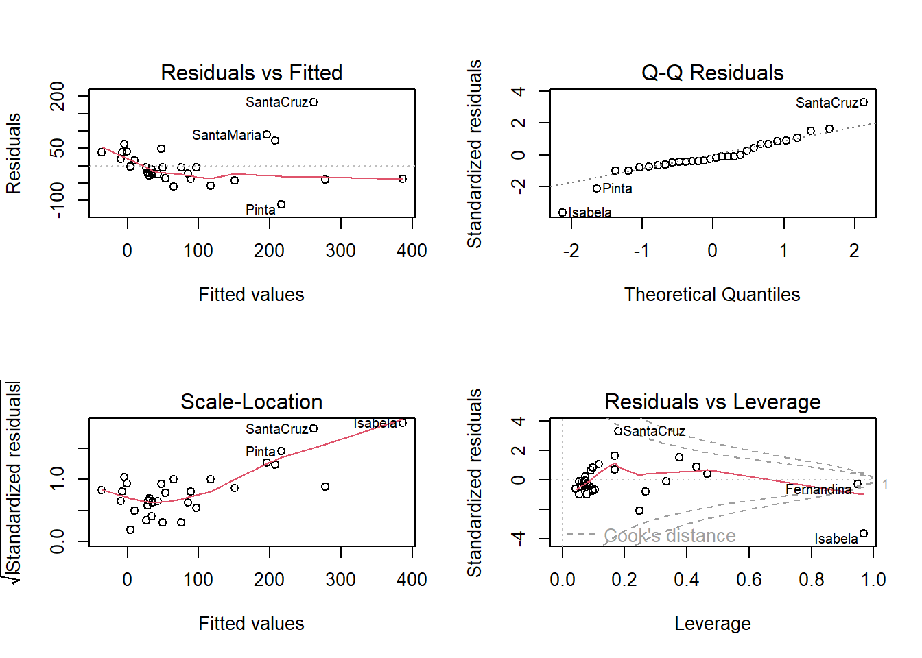
F-statistic:  15.7 on 5 and 24 DF,  p-value: 6.838e-07

Code

par(mfrow = c(2,2))
plot(lmod)

Warning in sqrt(crit * p * (1 - hh)/hh): NaNs produced

Warning in sqrt(crit * p * (1 - hh)/hh): NaNs produced

Code

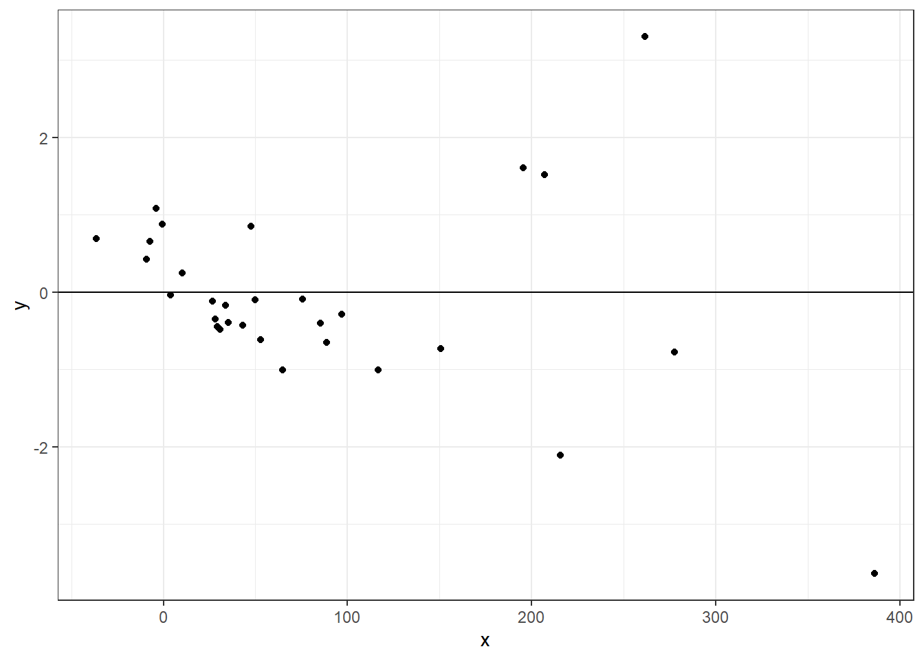
df = data.frame(x = fitted(lmod), y = stdres(lmod))
ggplot(df, aes(x = x, y = y)) + 
    geom_point() + 
    theme_bw() + 
    geom_hline(yintercept = 0)

Poisson Regression

Code

glmod = glm(Species ~ ., data = gala, family = poisson)
summary(glmod)


Call:
glm(formula = Species ~ ., family = poisson, data = gala)

Coefficients:
              Estimate Std. Error z value Pr(>|z|)    
(Intercept)  3.155e+00  5.175e-02  60.963  < 2e-16 ***
Area        -5.799e-04  2.627e-05 -22.074  < 2e-16 ***
Elevation    3.541e-03  8.741e-05  40.507  < 2e-16 ***
Nearest      8.826e-03  1.821e-03   4.846 1.26e-06 ***
Scruz       -5.709e-03  6.256e-04  -9.126  < 2e-16 ***
Adjacent    -6.630e-04  2.933e-05 -22.608  < 2e-16 ***
---
Signif. codes:  0 '***' 0.001 '**' 0.01 '*' 0.05 '.' 0.1 ' ' 1

(Dispersion parameter for poisson family taken to be 1)

    Null deviance: 3510.73  on 29  degrees of freedom
Residual deviance:  716.85  on 24  degrees of freedom
AIC: 889.68

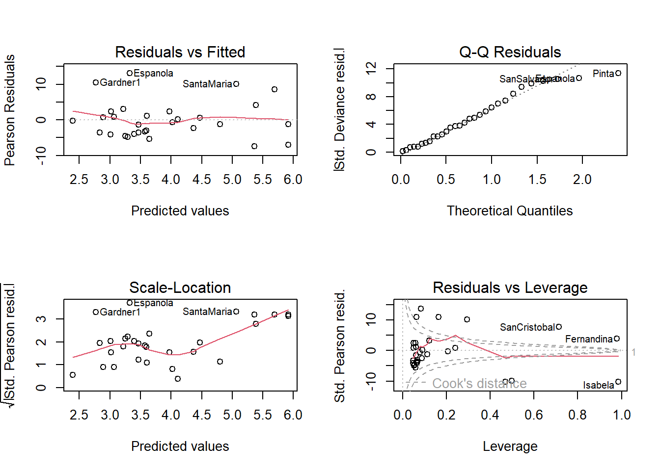
Number of Fisher Scoring iterations: 5

Code

par(mfrow = c(2,2)); plot(glmod)

Warning in sqrt(crit * p * (1 - hh)/hh): NaNs produced

Warning in sqrt(crit * p * (1 - hh)/hh): NaNs produced

Code

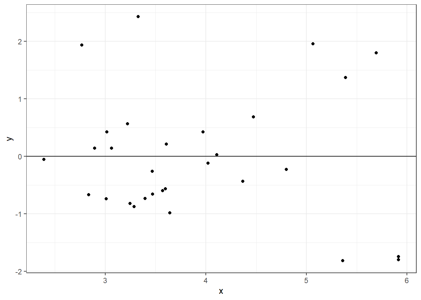
df = data.frame(x = predict(glmod, type = "link"), y = stdres(glmod))
ggplot(df, aes(x = x, y = y)) + 
    geom_point() + 
    theme_bw() + 
    geom_hline(yintercept = 0)

Interpret the parameter associated with Nearest

Code

exp(8.826e-03)

[1] 1.008865

This means that, given the model is correct, a one unit increase in Nearest is associated with a multiplicitive increase of \(e^{8.826e-03} = 1.01\) in species, on average, adjusting for other predictors.

Calculate the deviance for Poisson regression. Does this value show in the summary? Also, check the goodness of fit of this model using Pearson’s \(\chi^2\) statistic. What can you conclude about the fit?

Code

d_res <- with(gala,
              -2*sum(Species*log(fitted(glmod)/Species) - (Species - fitted(glmod))))
d_res

[1] 716.8458

Code

chisq_test <- with(gala, sum((Species - fitted(glmod))^2/fitted(glmod)))

pval <- 1 - pchisq(chisq_test, 24)
pval

[1] 0

Code

summary(glmod)


Call:
glm(formula = Species ~ ., family = poisson, data = gala)

Coefficients:
              Estimate Std. Error z value Pr(>|z|)    
(Intercept)  3.155e+00  5.175e-02  60.963  < 2e-16 ***
Area        -5.799e-04  2.627e-05 -22.074  < 2e-16 ***
Elevation    3.541e-03  8.741e-05  40.507  < 2e-16 ***
Nearest      8.826e-03  1.821e-03   4.846 1.26e-06 ***
Scruz       -5.709e-03  6.256e-04  -9.126  < 2e-16 ***
Adjacent    -6.630e-04  2.933e-05 -22.608  < 2e-16 ***
---
Signif. codes:  0 '***' 0.001 '**' 0.01 '*' 0.05 '.' 0.1 ' ' 1

(Dispersion parameter for poisson family taken to be 1)

    Null deviance: 3510.73  on 29  degrees of freedom
Residual deviance:  716.85  on 24  degrees of freedom
AIC: 889.68

Number of Fisher Scoring iterations: 5

The Chisq statistic is very large, and the p-value is small, so we would reject the null hypothesis that the model fits the data.

What do Prediction Look Like?

Let’s look at the binomial regression model for this.

Code

# predict admit from gre, gpa, rank
newData <- data.frame(gre=600, gpa=3.8, rank=as.factor(4))
predict(admission_glm, newdata = newData)

        1 
-1.127445

Code

predict(admission_glm, newdata = newData, type = 'response')

       1 
0.244633

Note that type response returns the percent associated with the model.

Side Note: type parameters in predict

response: default for many model types and returns the predicted values on the scale of the response variable
class: often used with classification models, this returns the predicted class label
terms: this returns the contribution of each term in the linear predictor to prediction
link: in GLMs, this returns the linear predictors, i.e. the predicted values on the scale of the linear predictor (before applying the link function)
prob: some models allow for returning a matrix of class probabilities, where each column corresponds to a class and each row corresponds to an observation
votes: for ensemble models, this might return a matrix of vote counts from different models