Generalized Addititive Models

Welcome to the world of GAMs and nonparametric regression.

Motivation

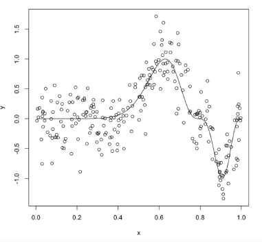
A parametric statistical model is a family of probability distributions with a finite set of parameters.

Example: The Normal Regression Model: \(Y \sim N(X\beta, \sigma^2I_n)\)

A parametric statistical model where the shape of predictors is determined by a function on a theoretical distribution (i.e. logarithmic, sigmoid, etc.)

A nonparametric function means that the shape of the predictor functions is determined by the data.

Suppose we have two individual predictors:

\(s(x_1)\): quadratic relationship with \(X_1\)
\(s(x_2)\): linear relationship with \(X_2\)

If we add these:

instead of using \(\eta = \beta_0 + \beta_1x_1 + \dots\) (glm setup)
we use the link function \(g(E[Y]) = \alpha + s_1(x_1) + s_2(x_2) + s_p(x_3)\), where:
- \(g\): link function
- \(Y\): response
- \(s_i\): different functions

Can be described as:

relationships between feature and response is not assumed to be linear
relationship between individual predictors and response are linear and nonlinear
we can estimate the relationship between the predictions and the response by simply adding up the individual features
nonparametric regression allows us to be more flexible with the form of \(f\) (i.e. in linear regression: \(f(x) = \beta_0 + \beta_1x_1 + \dots\))

Modeling

We learn \(f\) by assuming it comes from some smooth family of functions. In this case, the set of potential fits to the data is much larger than the parametric approach (i.e. linear line + quadratic + cubic). We can use kernel estimators for these types of data.

Advantages

flexibility
fewer distributional assumptions

Disadvantages

less efficient when structure of the relationship is available
interpretation difficulties

Marginal Impacts of Each Feature

defined as each feature’s individual relationship with response

Additive Function

model: \(Y_i = f(x_i) + \epsilon_i\)
\(k\): kernel
\(\lambda\): smoothing parameter

Additive Function

\[\hat{f_{\lambda}}(x) = \frac{\frac{1}{n\lambda}\sum\limits_{i=1}^n K(\frac{x-x_i}{\lambda})Y_i}{\sum\limits_{i=1}^n K(\frac{x-x_i}{\lambda})}\]

Smoothing Parameter

\(\lambda_{small}\): lots of wiggles
\(\lambda_{increases}\): less wiggles, more smoother, can find the “just right”
\(\lambda_{too large}\): too smooth, we risk missing key patterns
when choosing the smoothing parameter, pick the least smooth fit that does not show any implausible fluctuations
- GLMs: we know the link function we will use (identity, log, sigmoid)
- GAMs: we don’t know, they are learned from the data

Kernel Estimator

Kernel: a nonnegative, real-valued function \(K\) such that \(K(x) = K(-x)\) for all values of x (i.e. symmetry) and \(\int K(x) dx = 1\) (i.e. normalization).

Common Kernel Estimators

Uniform/Rectangular: \(K(x) = \frac{1}{2}\), \(-1 \leq x \leq 1\)
Gaussian/Normal: \(K(x) = \frac{1}{\sqrt{2\pi}} e^{-\frac{x^2}{2}}\)
Epanechnikov: \(K(x) = \frac{3}{4} (1-x)^2\), \(-1 \leq x \leq 1\)

Smoothing Splines

Given the model \(Y_i = f(x_i) + \epsilon_i\), we can choose \(\hat{f}\) by minimizing:

\(MSE = \frac{1}{n} \sum\limits_{i=1}^n (Y_i - f(x_i))^2\), or
\(\frac{1}{n} \sum\limits_{i=1}^n (Y_i - f(x_i))^2 + \lambda \int [f''(x)]^2dx\)

Smoothing vs. Regression Splines

Smoothing Splines

Smoothing splines are used to fit a smooth curve that passes close to the given datapoints.
They involve a roughness penalty to ensure the smoothness of the fitted curve. This penalty is an integrated squared second derivative times a smoothing parameter.
Smoothing splines typically have nkots at each data point, but the roughness penalty prevents overfitting by srhinking the coefficients.

Regression Splines

Regression splines fit a piecewise polynomial function with a reduced set of knots, compared to smoothing splines.
They do not use a roughness penalty. Instead, the fit is typically obtained by least squares, which minimizes the sum of squared residuals.
Regression splines are more about estimating functional relationships rather than transforming variables.

Main Differences

Smoothing splines are more flexible due to the roughness penalty, while regression splines provide a simpler model with fewer knots and no penalty term. Should be chosen specific for each analysis.

Implementation

Libraries

Code

library(tidyverse)
library(faraway)

Warning: package 'faraway' was built under R version 4.3.3

Code

library(sm)

Warning: package 'sm' was built under R version 4.3.3

Code

library(mgcv)

Kernel Models

Kernel Specific Data

Code

marketing = read.csv("https://raw.githubusercontent.com/bzaharatos/-Statistical-Modeling-for-Data-Science-Applications/master/Modern%20Regression%20Analysis%20/Datasets/marketing.txt", sep = "")
head(marketing)

  youtube facebook newspaper sales
1  276.12    45.36     83.04 26.52
2   53.40    47.16     54.12 12.48
3   20.64    55.08     83.16 11.16
4  181.80    49.56     70.20 22.20
5  216.96    12.96     70.08 15.48
6   10.44    58.68     90.00  8.64

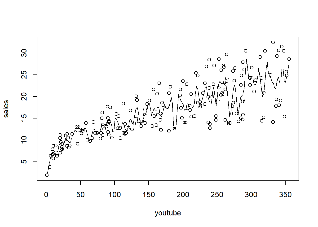
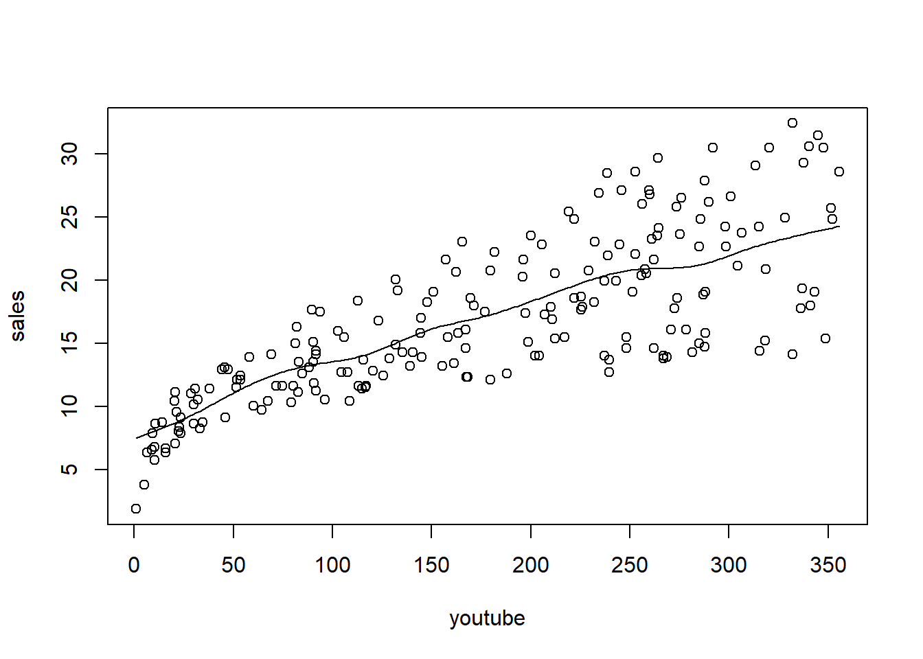
Plot sales (response) against youtube (predictor), and then fit and overlay a kernel regression

Kernel: normal
Smooth Parameter: 5

Code

with(marketing, plot(sales~youtube))
with(marketing, lines(ksmooth(youtube, sales, 'normal', 5)))

Kernel: normal
Smooth Parameter: 50

Code

with(marketing, plot(sales~youtube))
with(marketing, lines(ksmooth(youtube, sales, 'normal', 50)))

Measuring Kernel Performance

A function to calculate MSPE from a given parameter (bandwidth). Note that ordering the data is required.

Code

optimize_kernel <- function(train_set, test_set, response, predictor, bandwidth) {
    test_data <- test_set %>% select(!!sym(predictor), !!sym(response))
    test_data <- test_data %>% arrange(!!sym(predictor))
    obs <- test_data[[response]]
    preds <- ksmooth(x = train_set[[predictor]],
                     y = train_set[[response]],
                     'normal',
                     bandwidth,
                     x.points = test_set[[predictor]])$y
    mspe <- mean((obs - preds)^2)
    return(mspe)
}

Nonparametric Regressions

Create a sine wave dataset

Code

set.seed(88888)
n = 150
x = runif(n, 0, pi/2) 
y = sin(pi*x) + rnorm(n, 0, 0.5) 
plot(y ~ x, main = expression(f(x) == sin(pi*x)), pch = 16, cex=0.8, col = alpha("darkgrey", 0.9))

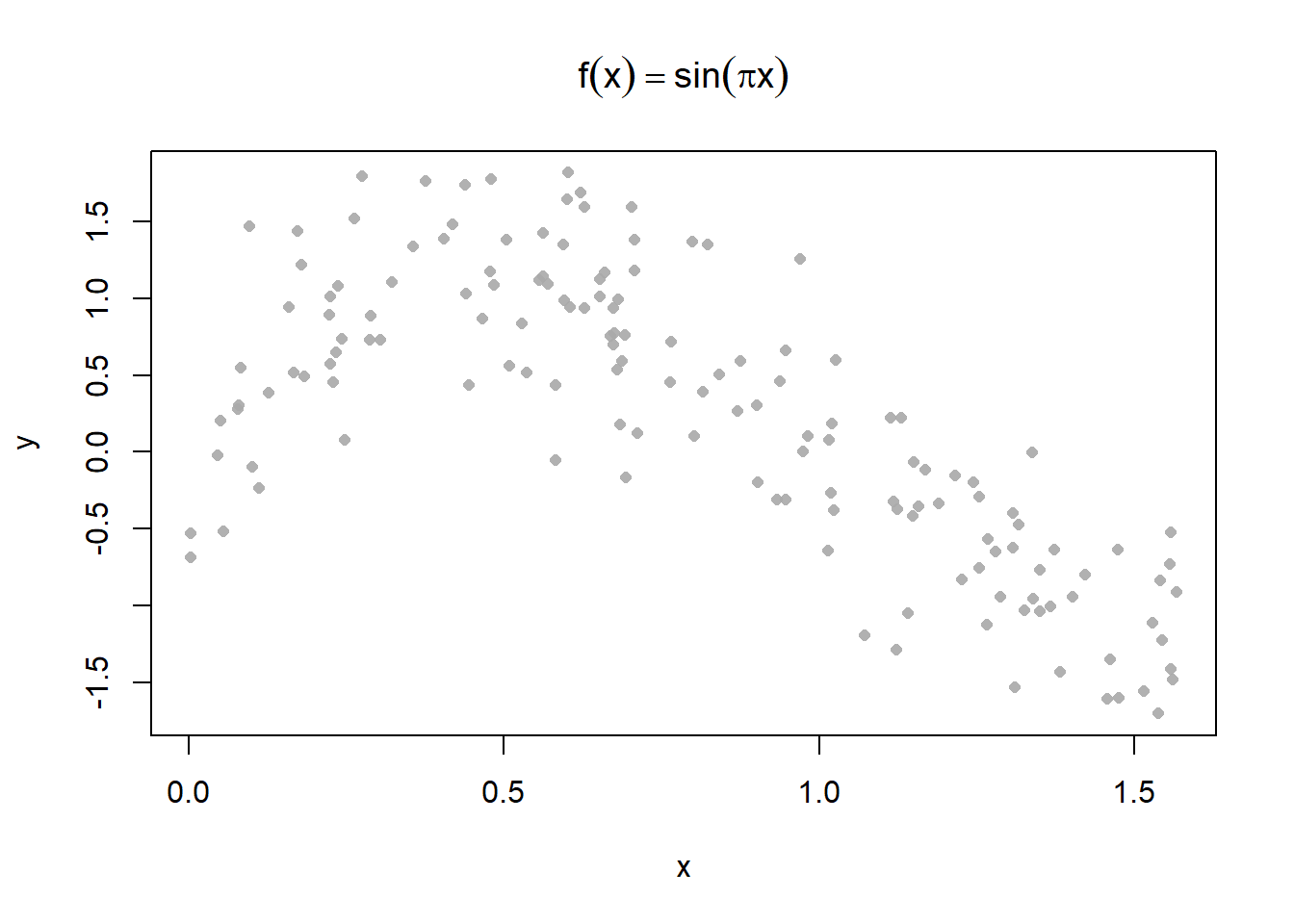
Plot some different kernel smoothing parameters

Code

plot(y ~ x, main = expression(f(x) == sin(pi*x)), pch = 16, cex=0.8, col = alpha("darkgrey", 0.9))
lines(ksmooth(x, y, "normal", 0.05))

Code

plot(y ~ x, main = expression(f(x) == sin(pi*x)), pch = 16, cex=0.8, col = alpha("darkgrey", 0.9))
lines(ksmooth(x, y, "normal", 1))

Code

plot(y ~ x, main = expression(f(x) == sin(pi*x)), pch = 16, cex=0.8, col = alpha("darkgrey", 0.9))
lines(ksmooth(x, y, "normal", 0.3))

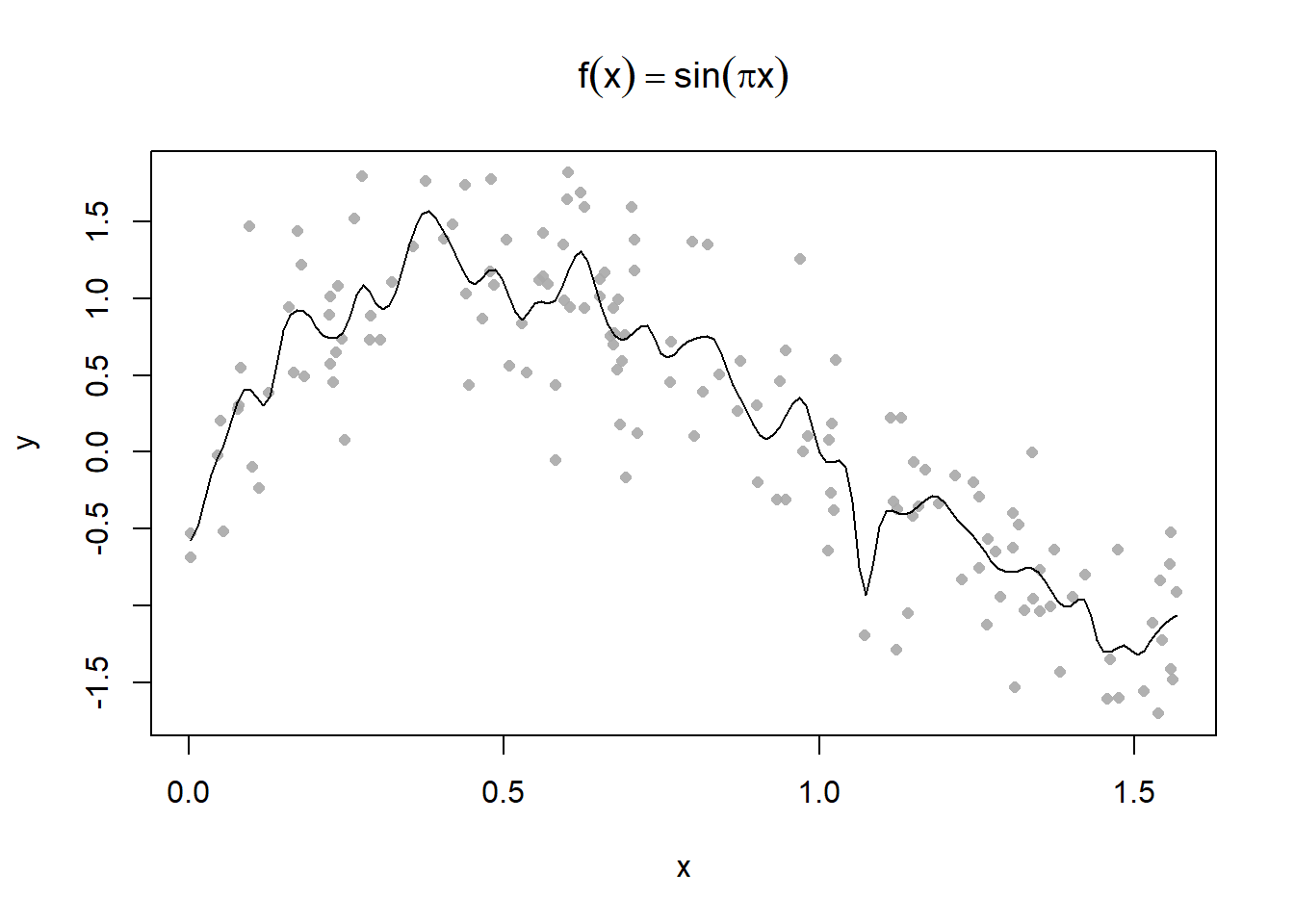
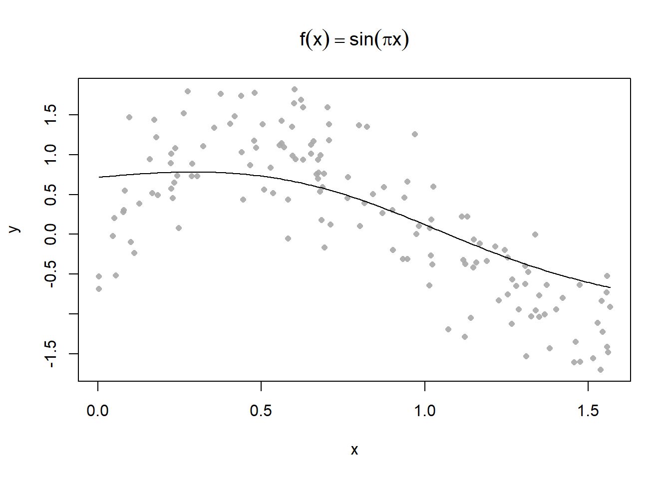
Use the 0.3 parameter to make some predictions

Code

ksmooth(x, y, "normal", 0.3, x.points = 0.5)

$x
[1] 0.5

$y
[1] 1.062831

Replicate `ksmooth` with a Custom Function

Code

# custom function
custom_smooth = function(x,y,lambda){
    f = matrix(NA, ncol = 1, nrow = length(x))
    for (i in 1:length(x)){
        f[i] = sum(dnorm((x-x[i])/lambda)*y)/sum(dnorm((x-x[i])/lambda))
    }
    s = data.frame(x[order(x)],f[order(x)])
    return(s)
}

# plotting with custom function
plot(y ~ x, main = expression(f(x) == sin(pi*x)), pch = 16, cex=0.8, col = alpha("darkgrey", 0.9))
s1 = custom_smooth(x, y, 0.1); 
s2 = custom_smooth(x,y, 0.2)
lines(s1$x,s1$f, type = "l", col = "blue")
lines(s2$x,s2$f, type = "l", col = "orange")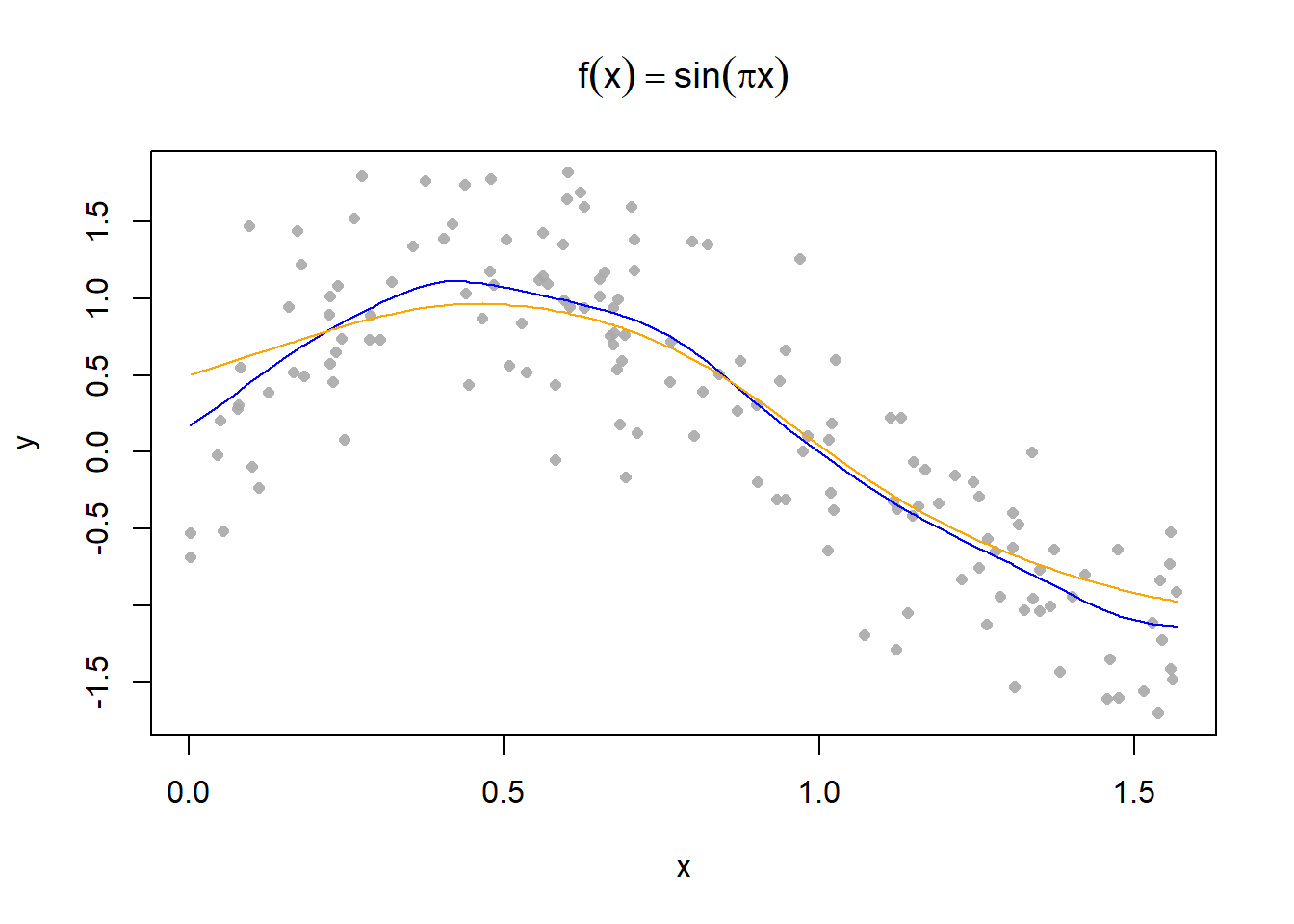

Smoothing Spline Estimator

Use smooth.spline where spar is the smoothing parameter.

Code

plot(y ~ x, main = expression(f(x) == sin(pi*x)), pch = 16, col = alpha("grey", 0.8))
lines(smooth.spline(x, y, spar = 0.5))

Code

plot(y ~ x, main = expression(f(x) == sin(pi*x)), pch = 16, col = alpha("grey", 0.8))
lines(smooth.spline(x, y, spar = 1))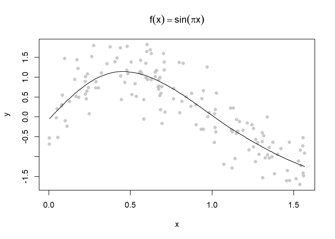

Implement Loess Fit

Use geom_smooth

Code

n = 50; x = runif(n, 0 , pi/2); y = sin(pi*x) + rnorm(n, 0, 2)
df = data.frame(x = x, y = y)
ggplot(df)+ 
geom_point(aes(x = x, y = y)) + 
geom_smooth(aes(x = x, y = y)) + 
theme_bw()

`geom_smooth()` using method = 'loess' and formula = 'y ~ x'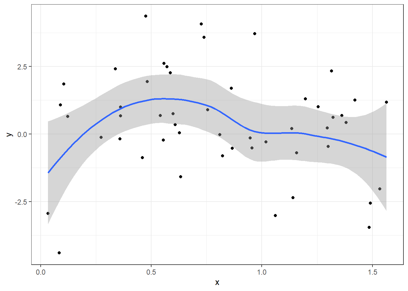

Other Non-Parametric Regressions and 3-d Plotting

Code

data(savings, package="faraway")
head(savings)

             sr pop15 pop75     dpi ddpi
Australia 11.43 29.35  2.87 2329.68 2.87
Austria   12.07 23.32  4.41 1507.99 3.93
Belgium   13.17 23.80  4.43 2108.47 3.82
Bolivia    5.75 41.89  1.67  189.13 0.22
Brazil    12.88 42.19  0.83  728.47 4.56
Canada     8.79 31.72  2.85 2982.88 2.43

sm package is for “Smoothing Methods for Nonparametric Regression and Density Estimation”

Code

# The savings rate will be our response variable
y = savings$sr
# pop15 and ddpi will be our two predictor variables
x = cbind(savings$pop15, savings$ddpi)

#sm.regression - usage: sm.regression(x, y, h, design.mat = NA, model = "none", weights = NA,
#group = NA, ...)
sm.regression(x,y,h=c(1,1),xlab="pop15",ylab="growth",zlab="savings rate")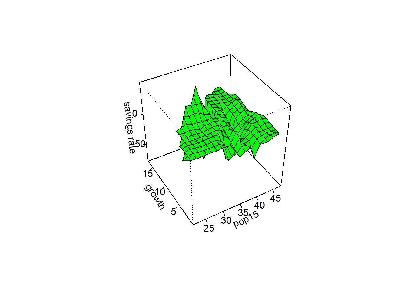

Code

sm.regression(x,y,h=c(5,5),xlab="pop15",ylab="growth",zlab="savings rate")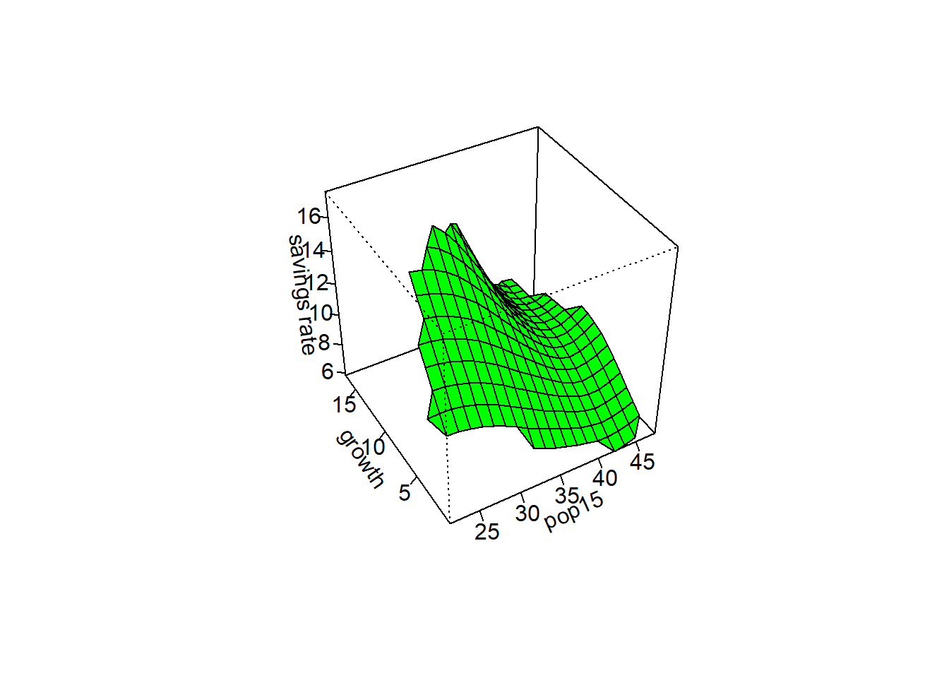

Produce a spline surface with the gam() Function

Code

amod = gam(sr ~ s(pop15,ddpi), data=savings)
vis.gam(amod, col="gray",ticktype="detailed",theta=-35)

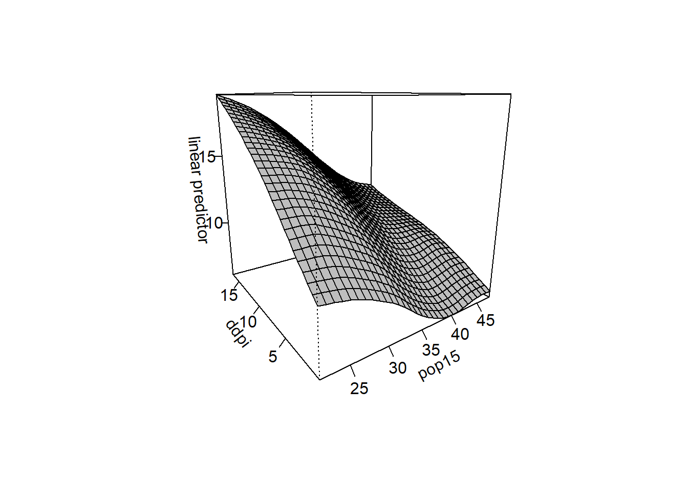
loess function

Code

lomod = loess(sr ~ pop15 + ddpi, data=savings)
xg = seq(21,48,len=20)
yg = seq(0,17,len=20)
zg = expand.grid(pop15=xg,ddpi=yg)
persp(xg,yg,predict(lomod,zg),theta=-35,ticktype="detailed",xlab="pop15",ylab="growth", zlab = "savings rate", col="gray")

GAMs

Code

data(exp)

Warning in data(exp): data set 'exp' not found

Code

head(exa)

       x       y m
1 0.0048 -0.0339 0
2 0.0086  0.1654 0
3 0.0117  0.0245 0
4 0.0170  0.1784 0
5 0.0261 -0.3466 0
6 0.0299 -0.7550 0

Code

plot(y ~ x, data = exa, main = "f(x) = sin^3(2pi x^2)")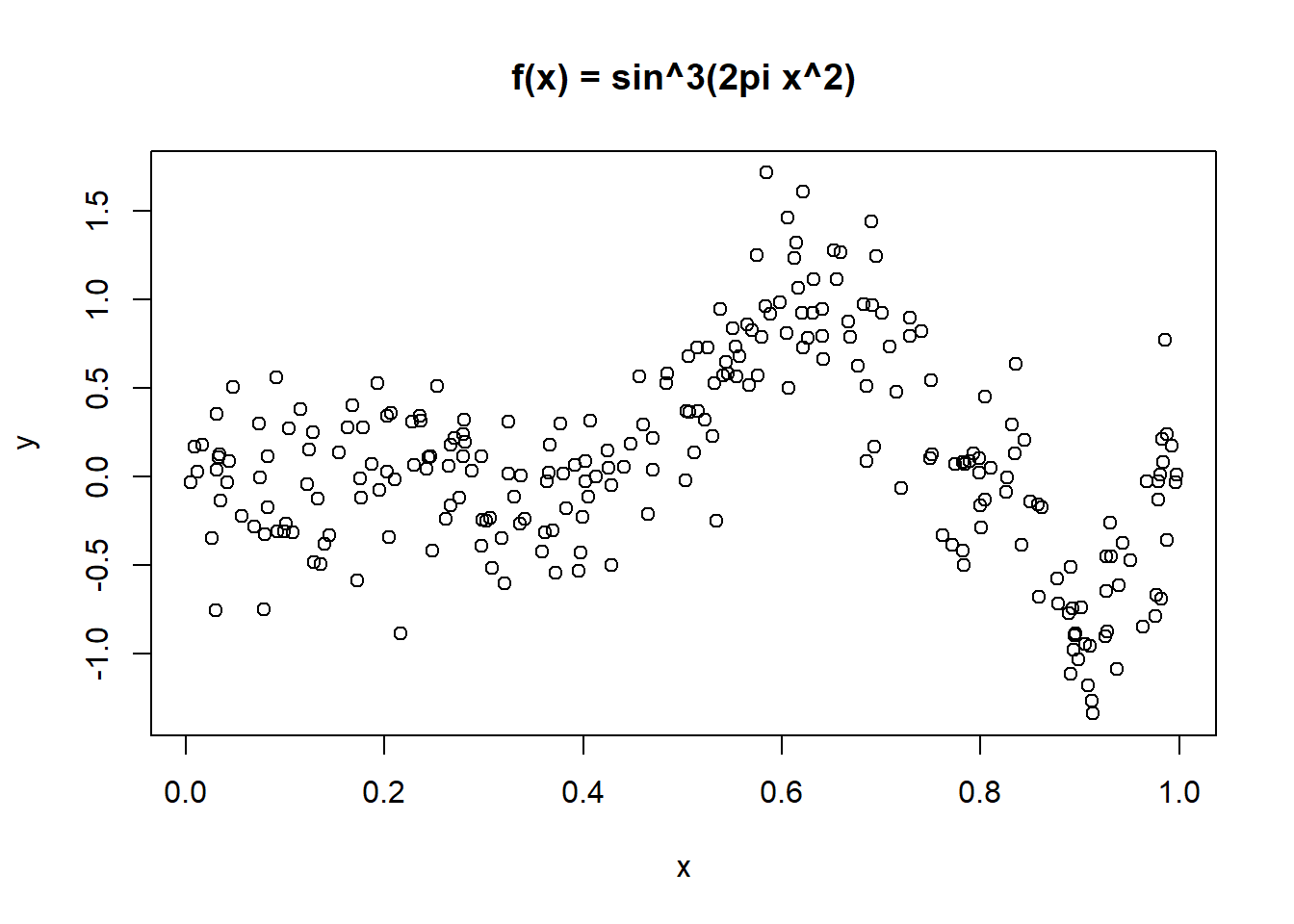

First, attempt a fit with kernel estimators of the unknown function \(Y = f(x)\).

Code

plot(y~x, data=exa, main="f(x) = sin^3(2*pi*x^2)")
lines(ksmooth(exa$x, exa$y, 'normal', 0.25))

Smoothing Spline vs. Regression Spline

Use a smoothing spline and a regression spline

Code

# default is spar=NULL
plot(y ~ x, data = exb, main = "f(x) = 0")
lines(smooth.spline(exb$x, exb$y))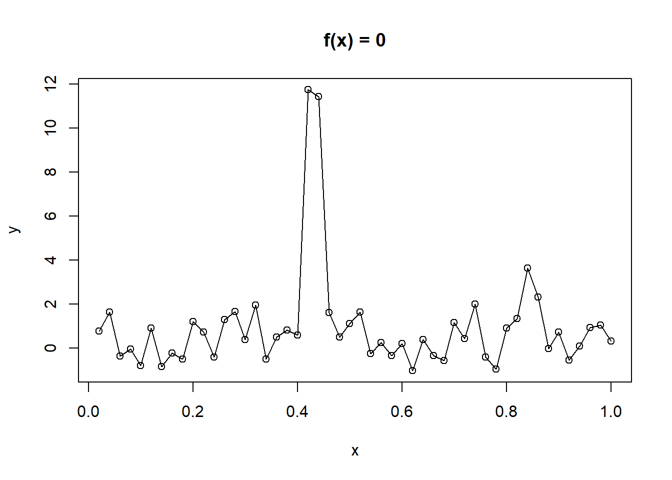

Code

plot(y ~ x, data = exb, main = "f(x) = 0")
lines(smooth.spline(exb$x, exb$y, spar = 1))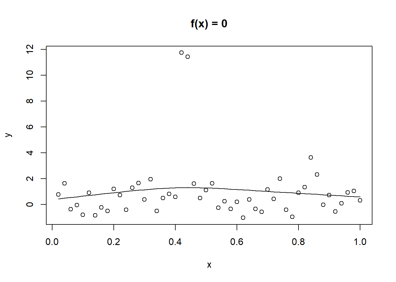

Simulated Data

Code

set.seed(12)

# construct predictors 
n <- 100
d <- data.frame(
    x1=rnorm(n, mean = 45, sd = 15),
    x2=sample(c('s','m','t'), size=n, replace=TRUE),
    x3=sample(c(F,T), size=n, replace=TRUE),
    stringsAsFactors=F)

head(d)

        x1 x2    x3
1 22.79149  t FALSE
2 68.65754  s  TRUE
3 30.64883  s FALSE
4 31.19992  s  TRUE
5 15.03537  t FALSE
6 40.91556  s FALSE

For this example, we make the response some nonlinear/nonparametric function of x1. In a realworld situation, we wouldn’t know this relationship and would estimate it. Other terms are modeled parametrically. The resposne has normal noise. The model we want is a Poisson GAM, with true relationship \(log(\mu_i) = \beta_1 + log(0.5x_i^2) - x_2 + x_3\)

Code

# make predictor
d$mu <- with(d, exp(log(0.5*x1^2)) - as.integer(as.factor(x2)) + as.integer(as.factor(x3)))
d$y <- rpois(n, d$mu) # manufacturing a poisson response

Code

mod_gam <- gam(y ~ s(x1) + as.integer(as.factor(x2)) + as.integer(as.factor(x3)), data=d, family=poisson)
mod_gam


Family: poisson 
Link function: log 

Formula:
y ~ s(x1) + as.integer(as.factor(x2)) + as.integer(as.factor(x3))

Estimated degrees of freedom:
8.64  total = 11.64 

UBRE score: -0.1023909

Code

summary(mod_gam)


Family: poisson 
Link function: log 

Formula:
y ~ s(x1) + as.integer(as.factor(x2)) + as.integer(as.factor(x3))

Parametric coefficients:
                          Estimate Std. Error z value Pr(>|z|)    
(Intercept)               6.798166   0.012954 524.799   <2e-16 ***
as.integer(as.factor(x2)) 0.001226   0.004055   0.302    0.762    
as.integer(as.factor(x3)) 0.003369   0.006704   0.503    0.615    
---
Signif. codes:  0 '***' 0.001 '**' 0.01 '*' 0.05 '.' 0.1 ' ' 1

Approximate significance of smooth terms:
        edf Ref.df Chi.sq p-value    
s(x1) 8.643  8.958  28056  <2e-16 ***
---
Signif. codes:  0 '***' 0.001 '**' 0.01 '*' 0.05 '.' 0.1 ' ' 1

R-sq.(adj) =  0.998   Deviance explained = 99.8%
UBRE = -0.10239  Scale est. = 1         n = 100

Code

plot(mod_gam)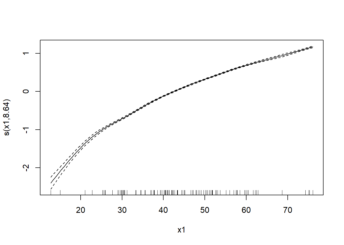

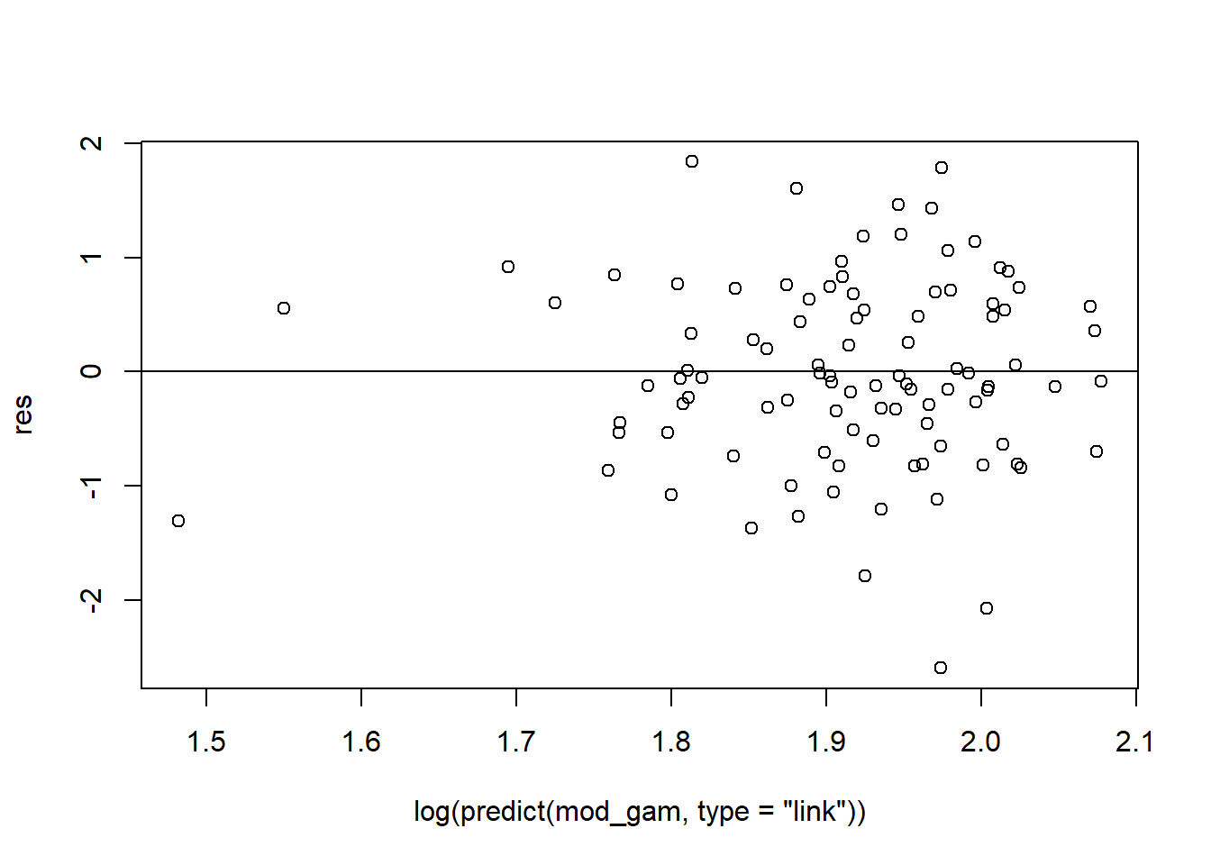
Code

res = residuals(mod_gam, response = 'deviance')
plot(log(predict(mod_gam, type = 'link')), res)
abline(h=0)

Code

gam.check(mod_gam)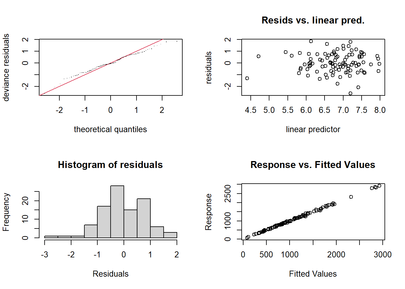


Method: UBRE   Optimizer: outer newton
full convergence after 8 iterations.
Gradient range [4.56651e-09,4.56651e-09]
(score -0.1023909 & scale 1).
Hessian positive definite, eigenvalue range [0.004773368,0.004773368].
Model rank =  12 / 12 

Basis dimension (k) checking results. Low p-value (k-index<1) may
indicate that k is too low, especially if edf is close to k'.

        k'  edf k-index p-value
s(x1) 9.00 8.64    1.02    0.51

Use GAMs on Another Dataset

Code

data(fat)
head(fat)

  brozek siri density age weight height adipos  free neck chest abdom   hip
1   12.6 12.3  1.0708  23 154.25  67.75   23.7 134.9 36.2  93.1  85.2  94.5
2    6.9  6.1  1.0853  22 173.25  72.25   23.4 161.3 38.5  93.6  83.0  98.7
3   24.6 25.3  1.0414  22 154.00  66.25   24.7 116.0 34.0  95.8  87.9  99.2
4   10.9 10.4  1.0751  26 184.75  72.25   24.9 164.7 37.4 101.8  86.4 101.2
5   27.8 28.7  1.0340  24 184.25  71.25   25.6 133.1 34.4  97.3 100.0 101.9
6   20.6 20.9  1.0502  24 210.25  74.75   26.5 167.0 39.0 104.5  94.4 107.8
  thigh knee ankle biceps forearm wrist
1  59.0 37.3  21.9   32.0    27.4  17.1
2  58.7 37.3  23.4   30.5    28.9  18.2
3  59.6 38.9  24.0   28.8    25.2  16.6
4  60.1 37.3  22.8   32.4    29.4  18.2
5  63.2 42.2  24.0   32.2    27.7  17.7
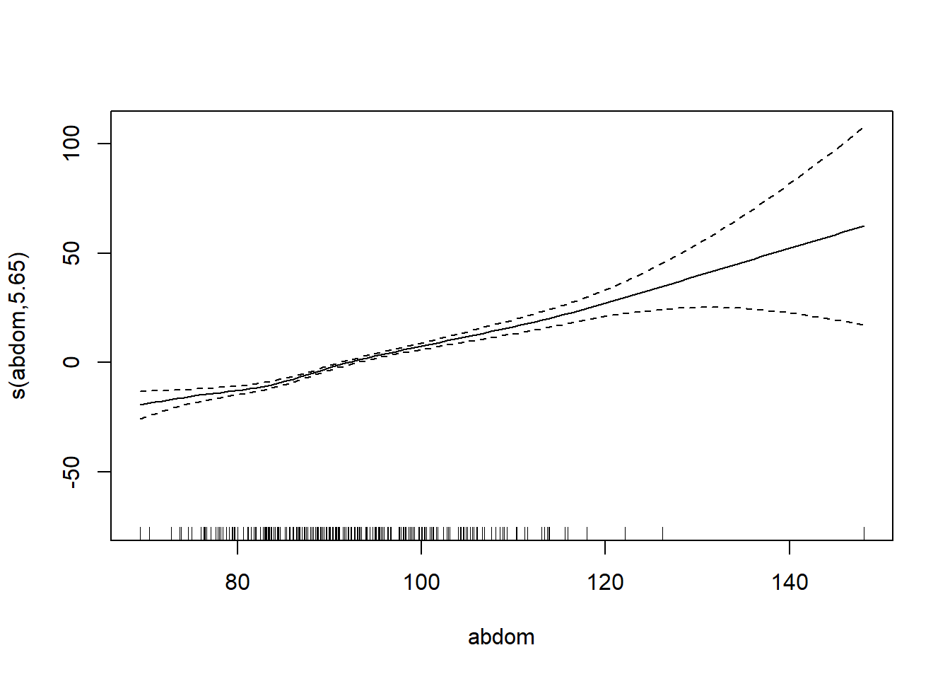
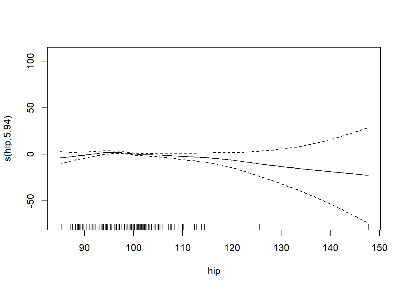
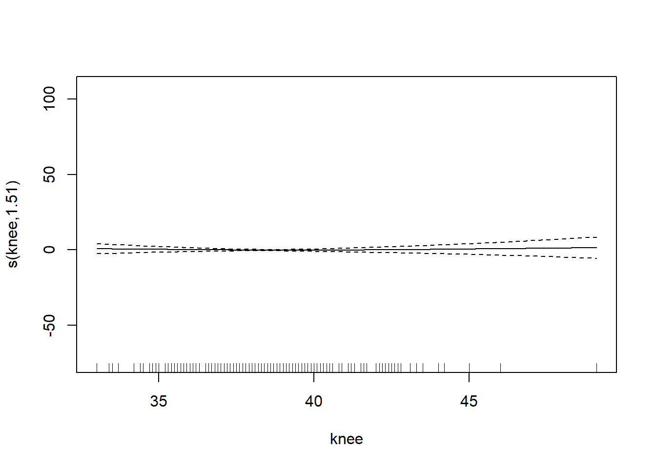
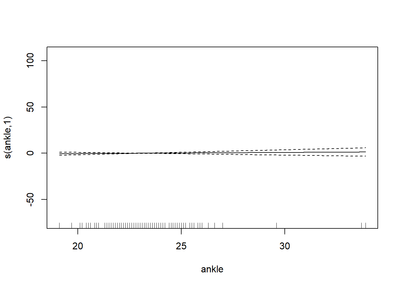
6  66.0 42.0  25.6   35.7    30.6  18.8

Code

# want to determining if we should use the smoothing function on each of the features
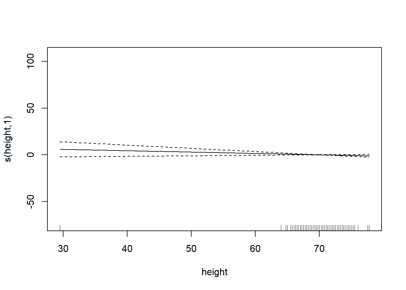
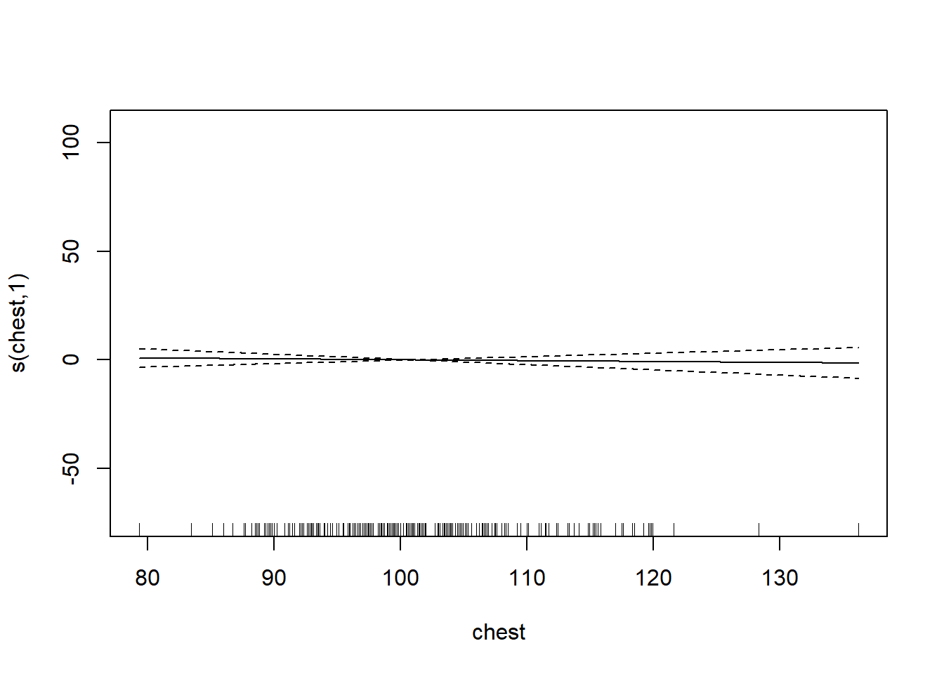
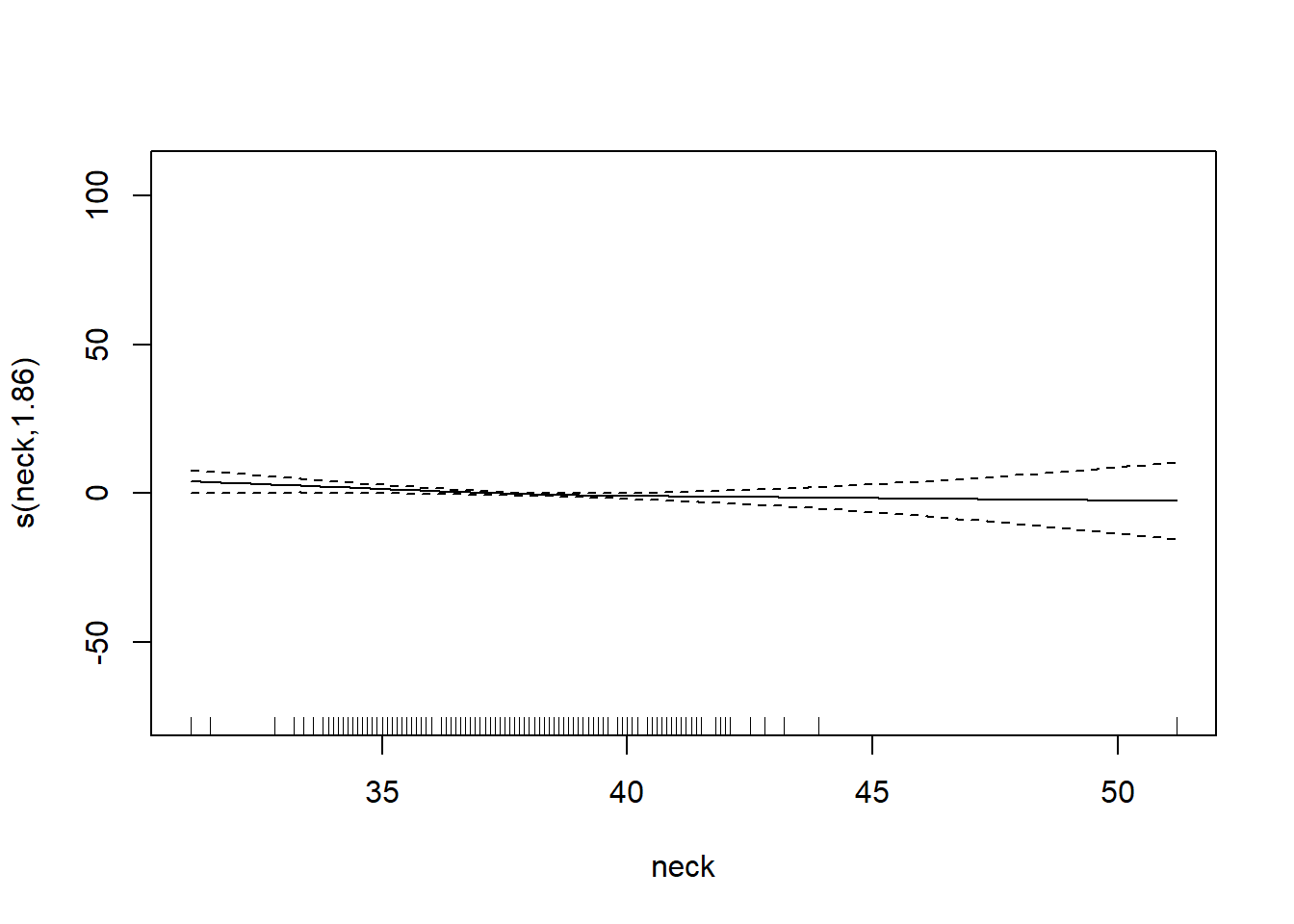
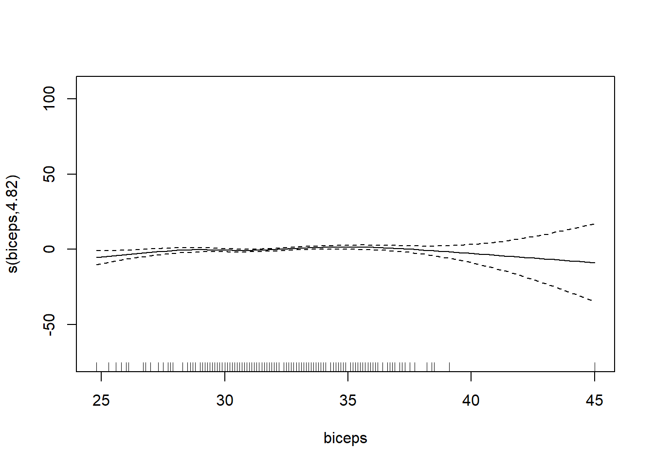
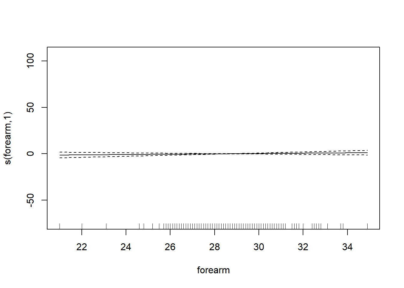
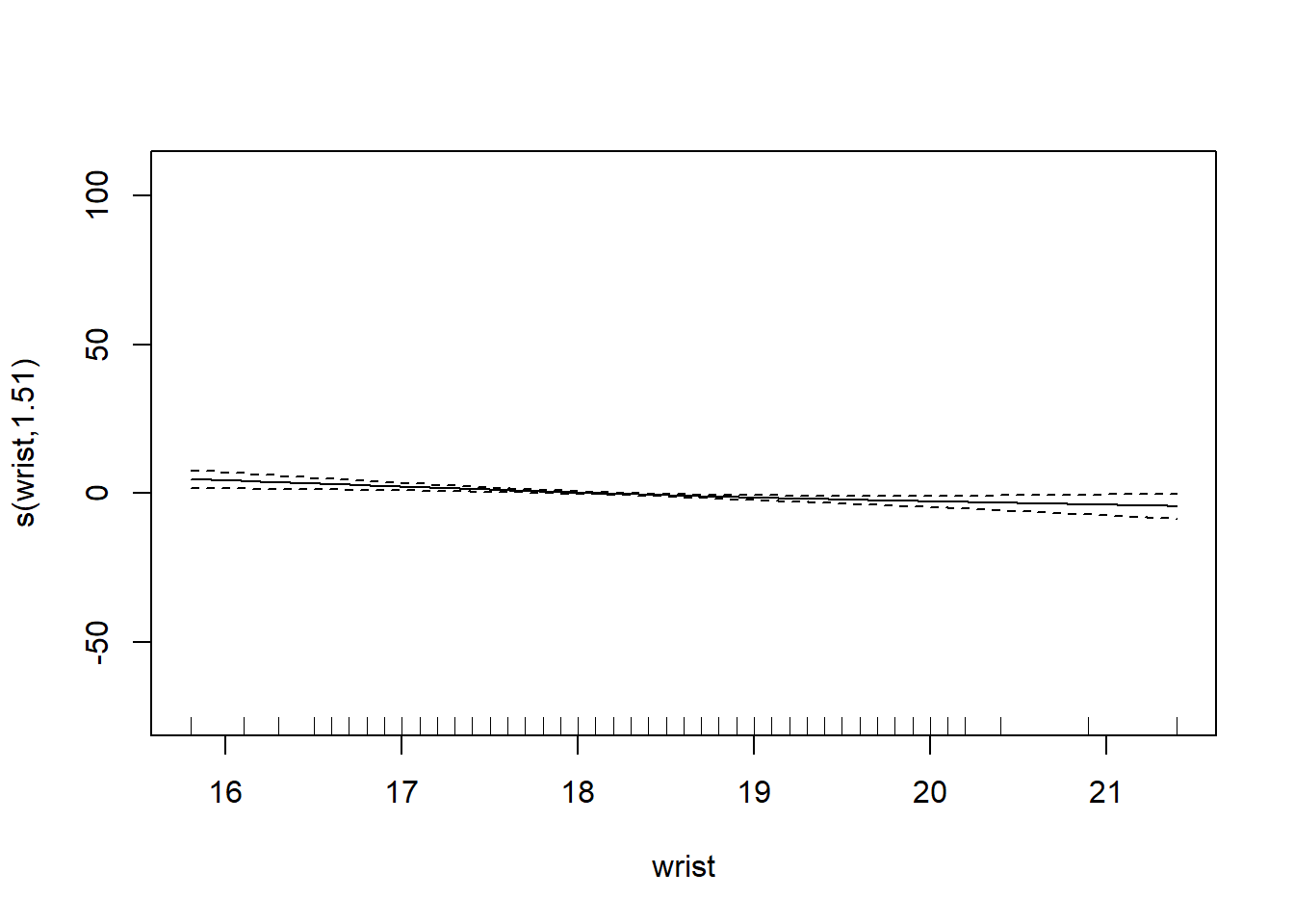
gam_mod <- gam(siri ~ s(weight) + s(height) + s(chest) + s(neck) + s(abdom) + s(hip) + s(thigh) + s(knee) + s(ankle) + s(biceps) + s(forearm) + s(wrist), data=fat)

# res vs predicted
res <- residuals(gam_mod, type='deviance')
plot(log(predict(gam_mod, type='response')), res)
abline(h=0)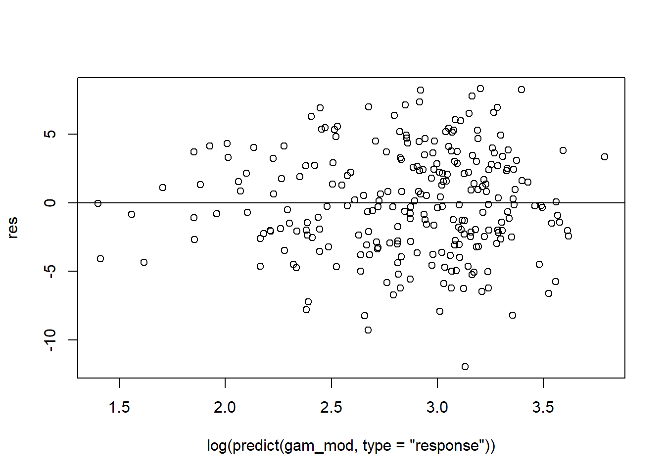

Code

# qqplot
qqnorm(res)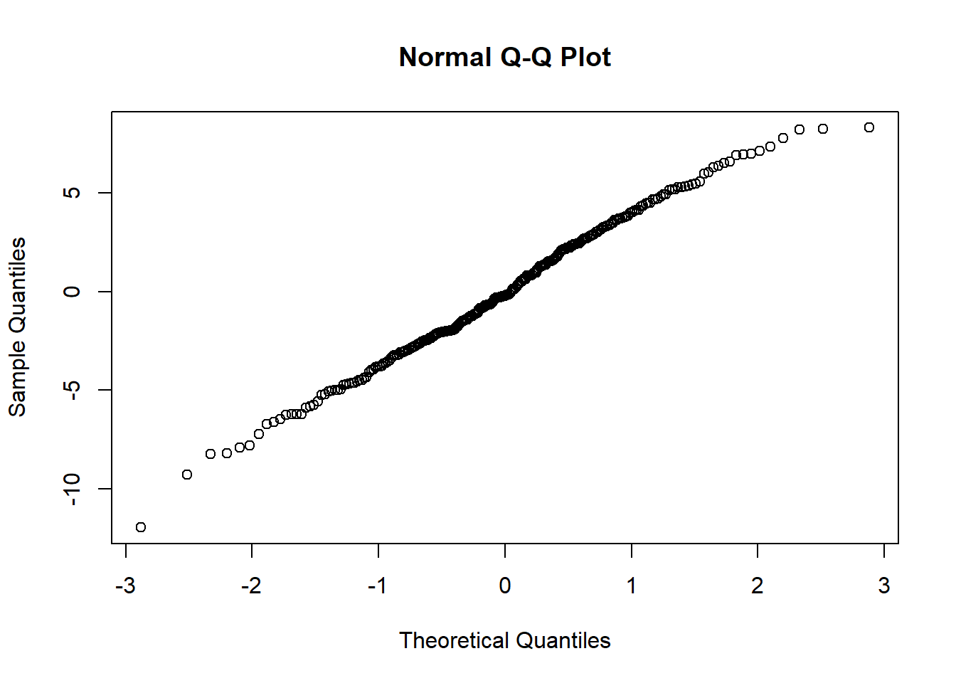

Code

# missed a plot - SEE LECTURE VERSION
# maybe
plot.gam(gam_mod)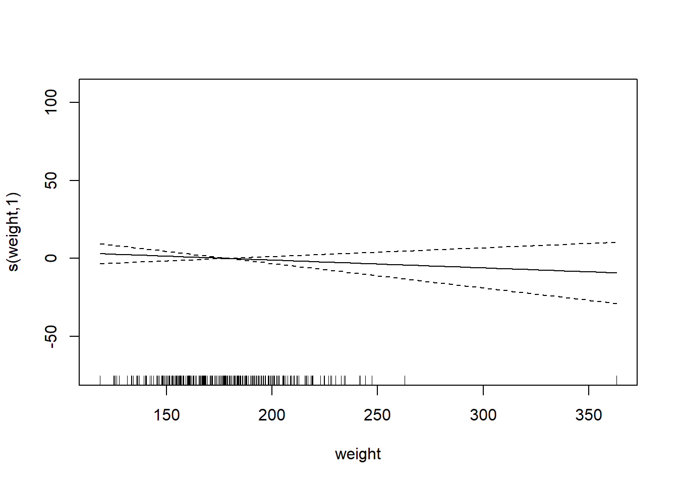

Code

data(ozone)
head(ozone)

  O3   vh wind humidity temp  ibh dpg ibt vis doy
1  3 5710    4       28   40 2693 -25  87 250  33
2  5 5700    3       37   45  590 -24 128 100  34
3  5 5760    3       51   54 1450  25 139  60  35
4  6 5720    4       69   35 1568  15 121  60  36
5  4 5790    6       19   45 2631 -33 123 100  37
6  4 5790    3       25   55  554 -28 182 250  38

Code

gam_ozone <- gam(O3 ~ s(temp) + s(ibh) + s(ibt), data=ozone)
summary(gam_ozone)


Family: gaussian 
Link function: identity 

Formula:
O3 ~ s(temp) + s(ibh) + s(ibt)

Parametric coefficients:
            Estimate Std. Error t value Pr(>|t|)    
(Intercept)  11.7758     0.2382   49.44   <2e-16 ***
---
Signif. codes:  0 '***' 0.001 '**' 0.01 '*' 0.05 '.' 0.1 ' ' 1

Approximate significance of smooth terms:
          edf Ref.df      F  p-value    
s(temp) 3.386  4.259 20.681  < 2e-16 ***
s(ibh)  4.174  5.076  7.338 1.74e-06 ***
s(ibt)  2.112  2.731  1.400    0.214    
---
Signif. codes:  0 '***' 0.001 '**' 0.01 '*' 0.05 '.' 0.1 ' ' 1

R-sq.(adj) =  0.708   Deviance explained = 71.7%
GCV = 19.346  Scale est. = 18.72     n = 330

Code

plot.gam(gam_ozone)

Note: IBT has evidence that it could be linear, while others do not. What we want to see here is a linear line through the confidence bounds.

Motivation

Modeling

Advantages

Disadvantages

Marginal Impacts of Each Feature

Additive Function

Smoothing Parameter

Kernel Estimator

Smoothing Splines

Smoothing vs. Regression Splines

Implementation

Kernel Models

Measuring Kernel Performance

Nonparametric Regressions

Replicate ksmooth with a Custom Function

Smoothing Spline Estimator

Implement Loess Fit

Other Non-Parametric Regressions and 3-d Plotting

GAMs

Smoothing Spline vs. Regression Spline

Simulated Data

Use GAMs on Another Dataset

Replicate `ksmooth` with a Custom Function