Frequent Patterns

Association Rules

We’re trying to find frequent itemsets given a list of sets. Essentially, finding the subsets within these sets that are commonly together.

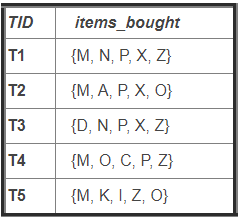
Two prime examples of this are items purchased in transactions and movies watched in a library.

The Basics

Support

Support quantifies how often an itemset appears in a dataset (proportion).

Let \(I\) be an itemset, then:

\(Support(I) = \frac{\text{number of sets containing } I}{\text{total number of sets}}\)

Suppose we have 100 customer’s movie watchlists, and we’re interested in making association rules surrounding movie \(M\).

We know that movie (or movie set) \(M\) is in 10 of the watchlists.

\(Support(M) = \frac{10}{100}\)

Additionally, we could have support for an association rule (\(Support(A \rightarrow C)\)), where \(A\) is the antecendent and \(C\) is the consequent (both are itemsets), which would look like:

\(Support(A \rightarrow C) = \frac{\text{number of sets containing } A \text{ and } C}{\text{total number of sets}}\)

Confidence

Confidence quantifies the likelihood an itemset’s consequent occurs given its antecent (i.e. the probability a consequent occurs given its antecent).

Let \(A\) be an itemset’s antecent and \(C\) be an itemset’s consequent, then:

\(Confidence(A \rightarrow C) = \frac{\text{proportion of sets containing} A \text{ and } C }{\text{proportion of sets containing} A}\)

Note that the concept of confidence is roughly derived with the help of the concept of conditional probability.

\(Confidence(A \rightarrow C) = P(C|A) = \frac{P(C, A)}{P(A)}\)

A key difference is that the numerator is is not a true intersection of events, but it contains the every element in itemsets \(A\) and \(C\). It’s more clear to use the respective definitions of support here.

\(Confidence(A \rightarrow C) = \frac{Support(A \cup C)}{Support(A)}\)

Suppose we want to recommend a movie (or movie set), \(M_2\), and we’re creating rules based on those who have watched the movie (or movie set) \(M_2\).

\(Confidence(M_1 \rightarrow M_2) = \frac{\text{proportion of watchlists containing} M_1 \text{ and } M_2} {\text{proportion of watchlists containing} M_1}\)

\(= \frac{Support(M_1 \cup M_2)}{Support(M_1)}\)

Lift

Lift assesses the performance of an association rule by quantifying an improvement (or degradation) from the initial prediction, where the initial prediction would be the support of the antecent.

\(Lift(C \rightarrow A) = \frac{Confidence(A \rightarrow C)}{Support(C)}\)

\(= \frac{\frac{Support(A \cup C)}{Support(A)}}{Support(C)}\)

\(= \frac{Support(A \cup C)}{Support(A)Support(C)}\)

Suppose we have a rule suggesting we recommend a movie (or movie set), \(M_2\), to those have seen movie(s) \(M_1\) (i.e. \(M_1 \rightarrow M_2\)).

We gather the following measurements:

• \(Support(M_1) = P(M_1) = 0.4\)
• \(Support(M_2) = P(M_2) = 0.1\)
• \(Confidence(M_1 \rightarrow M_2) = \frac{Support(M_1 \cup M_2)}{Support(M_1)} = 0.175\)
• \(Lift(M_1 \rightarrow M_2) = \frac{Confidence(M_1 \rightarrow M_2)}{Support(M_2)} = 1.75\)

How to Interpret Lift

Because \(lift((M_1 \rightarrow M_2)) > 1\), this rule provides evidence that the suggesting \(M_2\) to those who have have seen \(M_1\) is better than just suggesting \(M_2\).

In general, this yields the result that if \(lift > 1\), the association rule improves our initial prediction.

Maximal Itemset

Maximal Itemset: itemset in which none of its supersets are frequent.

Closed Itemset

Closed Itemset: itemset in which none of its immediate supersets have the same support count as the itemset, itself.

k-itemset

k-itemset: itemset which contains k items.

When finding frequencies, can refer to each sized frequency set as n-frequent, where n is the number of items in an itemset (or subset).

Apriori Property

Apriori Property: all non-empty subsets of frequent itemsets must be frequent.

Given a frequent itemset, all non-empty subsets of the frequent itemset are frequent as well.

Antimonotonicity

Antimonotonicity: If a set cannot pass a test, all its supersets will fail the test as well.

Roughly the contrapositive of the Apriori Property for association rules.

If an itemset is infrequent, all its supersets will be infrequent as well.

Maximum Number of of Possible Frequent itemsets (excluding the emptyset)

\(2^n - 1\), where \(n\) is the total number of items in the dataset. This is actually problematic due to the factorial growth per element.

For example, take a frequent itemset with just 100 elements. The total number of frequent itemsets that it contains is:

\(\sum\limits_{n = 1}^{1000}{100 \choose n} = 2^{100} - 1 \approx 1.27 x 10^{30}\)

The Apriori Algorithm

Suppose we have a list of itemsets (i.e. transactions), and we would like a systematic method to find the strong association rules from this list (i.e. find all the rules constrained to a given a minimum support and confidence). The Apriori Algorithm uses the Apriori pruning principal to construct these level-wise subsets in a progressive manner.

Outline

The key steps of the Apriori Algorithm follow this computation process: - initial iteration: count number of occurrences of each item to form candidate 1-itemsets, \(C_1\) - initial minimum support check: compare \(C_1\) with the minimum support, removing any occurrence which does not pass the minimum support test, to form frequent 1-itemsets, \(L_1\) - future iterations: form candidate k-itemsets, \(C_k\) where \(k > 1\) - join \(L_{k-1}\) with itself such that all permutations are formed with length of \(k\) - future iterations: form frequent k-itemsets, \(L_k\) where \(k > 1\) - compare \(C_k\) with the minimum support, removing any occurrence which does not pass the minimum support test - repeat until maximum transaction length from dataset or no candidate or frequent itemsets can be generated

Note that by the Apriori pincipal that all non-empty subsets of the frequent itemset are frequent as well, we can report the final \((k+1)\)-length frequent itemsets, as those contain the non-empty frequent itemsets.

Implementation

Custom Example

from itertools import permutations
def custom_apriori(transaction_dict, min_sup = 0.5):
    # get all unique items in transactions
    freq_items = set()
    for transaction in transaction_dict:
        freq_items = freq_items.union(transaction_dict[transaction])
        
    # begin with frequent k=1 itemsets
    # boolean initialized to true for meeting support, will exit when false
    # initialize frequency dictionary to store results
    meets_support = True
    k = 1
    frequency_dict = {}
    
    while meets_support:
        # create list for each permutation, initializing support count at 0
        prev_perms = []
        candidate = []
        for perm in permutations(freq_items, k):
            # prevent duplicates since order doesn't matter
            if set(perm) not in prev_perms:
                candidate.append([set(perm), 0])
                prev_perms.append(set(perm))

        # loop through each permutation in candidate
        # if the intersection of the permutation with a transaction is the permutation
        # then that indicates it is an itemset within the transaction
        for itemset in candidate:
            for transaction in transaction_dict:
                if itemset[0].intersection(transaction_dict[transaction]) == itemset[0]:
                    itemset[1] += 1
        # keep the permutations with support count at least at the minimum support
        frequency = [itemset[0] for itemset in candidate if (itemset[1] / len(transaction_dict)) >= min_sup]
        # if the frequency list is empty, there are no more permutations which can meet the minimum support threshold
        # we can exit it at that case due to antimonotonicity
        if len(frequency) != 0:
            # add to frequency dictionary for each round
            frequency_dict[k] = frequency
            # extract unique items from new frequency itemsets
            freq_items = set()
            for itemset in frequency:
                freq_items = freq_items.union(itemset)
            k += 1
            
        else:
            meets_support = False
            
    return frequency_dict

Suppose we were given the example of

transaction_dict = {'t1': {'M', 'N', 'P', 'X', 'Z'},
                    't2': {'M', 'A', 'P', 'X', 'O'},
                    't3': {'D', 'N', 'P', 'X', 'Z'},
                    't4': {'M', 'O', 'C', 'P', 'Z'},
                    't5': {'M', 'K', 'I', 'Z', 'O'}}

A quick aside on the number of datasets:

\(2^n - 1 = 2^{11} - 1 = 2047\) possible frequent itemsets.

The results of the Custom Apriori Algorithm will produce:

custom_apriori(transaction_dict)

{1: [{'X'}, {'M'}, {'O'}, {'Z'}, {'P'}],
 2: [{'M', 'O'}, {'P', 'X'}, {'M', 'Z'}, {'M', 'P'}, {'P', 'Z'}]}

Note that we’re not giving the interim support counts or the final support counts, how about we take a look at a widely used and accepted module.

The mlxtend Library

Import the following from mlxtend:

# libraries
import numpy as np
import pandas as pd
from mlxtend.preprocessing import TransactionEncoder
from mlxtend.frequent_patterns import apriori as ml_apriori
from mlxtend.frequent_patterns import association_rules as ml_association

For the TransactionEncoder, we’re going to want the transactions in a list of lists:

# turn transactions into list of lists
transactions = [list(transaction_dict[transaction]) for transaction in  transaction_dict]

Encode the transactions list:

# put the transactions' lists in a boolean dataframe format
con = TransactionEncoder()
con_arr = con.fit(transactions).transform(transactions)
df_transformed = pd.DataFrame(con_arr, columns = con.columns_)

Run the algorithm:

# mlxtend apriori function
dataset_apriori = ml_apriori(df_transformed, use_colnames = True, min_support = 0.5)
dataset_apriori

	support	itemsets
0	0.8	(M)
1	0.6	(O)
2	0.8	(P)
3	0.6	(X)
4	0.8	(Z)
5	0.6	(O, M)
6	0.6	(P, M)
7	0.6	(M, Z)
8	0.6	(P, X)
9	0.6	(P, Z)

And then extending past the frequent itemset results, we can run a function which will return association rules:

# mlxtend association rules to display the rules with a 50% minimum threshold on the frequent itemsets (dataset_apriori)
rules = ml_association(dataset_apriori, metric = 'confidence', min_threshold = 0.50)
rules

	antecedents	consequents	antecedent support	consequent support	support	confidence	lift	leverage	conviction	zhangs_metric
0	(O)	(M)	0.6	0.8	0.6	1.00	1.2500	0.12	inf	0.50
1	(M)	(O)	0.8	0.6	0.6	0.75	1.2500	0.12	1.6	1.00
2	(P)	(M)	0.8	0.8	0.6	0.75	0.9375	-0.04	0.8	-0.25
3	(M)	(P)	0.8	0.8	0.6	0.75	0.9375	-0.04	0.8	-0.25
4	(M)	(Z)	0.8	0.8	0.6	0.75	0.9375	-0.04	0.8	-0.25
5	(Z)	(M)	0.8	0.8	0.6	0.75	0.9375	-0.04	0.8	-0.25
6	(P)	(X)	0.8	0.6	0.6	0.75	1.2500	0.12	1.6	1.00
7	(X)	(P)	0.6	0.8	0.6	1.00	1.2500	0.12	inf	0.50
8	(P)	(Z)	0.8	0.8	0.6	0.75	0.9375	-0.04	0.8	-0.25
9	(Z)	(P)	0.8	0.8	0.6	0.75	0.9375	-0.04	0.8	-0.25

The FP-Growth Algorithm

Partitioning

• A frequent itemset must be frequent in at least one partition
• If an itemset is not frequent in all partitions, we can ignore it
• Using this, we can divide and conquer by addressing the following:
  • What is the size of each partition?
  • What is the number of partitions?

The partitioning method takes two data scans.

Implementation

FP-Growth uses hash-trees to find frequent itemsets with candidate generation as mining long patterns needs many scans and generates a lot of candidates. It helps avoid common bottlenecks such as candidate generation and candidate tests.

FP Tree Construction

1. Scan and find frequent 1-itemset (given a minimum support)
2. Sort the frequent 1-itemset in descending order
3. Scan and construct the FP-tree
4. Find conditional pattern base

The mlxtend Library

Import New Library for FP-Growth.

# libraries
import numpy as np
import pandas as pd
from mlxtend.preprocessing import TransactionEncoder
from mlxtend.frequent_patterns import apriori as ml_apriori
from mlxtend.frequent_patterns import association_rules as ml_association
# new function for fp-growth
from mlxtend.frequent_patterns import fpgrowth as ml_fpgrowth

We use the same initialization process as above.

transactions

[['X', 'N', 'M', 'Z', 'P'],
 ['O', 'X', 'M', 'A', 'P'],
 ['D', 'X', 'N', 'Z', 'P'],
 ['O', 'M', 'Z', 'C', 'P'],
 ['O', 'I', 'M', 'Z', 'K']]

con = TransactionEncoder()
con_arr = con.fit(transactions).transform(transactions)
df_transformed = pd.DataFrame(con_arr, columns = con.columns_)
df_transformed

	A	C	D	I	K	M	N	O	P	X	Z
0	False	False	False	False	False	True	True	False	True	True	True
1	True	False	False	False	False	True	False	True	True	True	False
2	False	False	True	False	False	False	True	False	True	True	True
3	False	True	False	False	False	True	False	True	True	False	True
4	False	False	False	True	True	True	False	True	False	False	True

Frequent Itemsets through Apriori

# frequent itemsets through apriori
dataset_apriori = ml_apriori(df_transformed, use_colnames = True, min_support = 0.5)
dataset_apriori

	support	itemsets
0	0.8	(M)
1	0.6	(O)
2	0.8	(P)
3	0.6	(X)
4	0.8	(Z)
5	0.6	(O, M)
6	0.6	(P, M)
7	0.6	(M, Z)
8	0.6	(P, X)
9	0.6	(P, Z)

Frequent Itemsets through FP-Growth

# frequent itemsets through fp-growth
dataset_fpgrowth = ml_fpgrowth(df_transformed, use_colnames = True, min_support = 0.5)
dataset_fpgrowth

	support	itemsets
0	0.8	(Z)
1	0.8	(P)
2	0.8	(M)
3	0.6	(X)
4	0.6	(O)
5	0.6	(P, Z)
6	0.6	(P, M)
7	0.6	(M, Z)
8	0.6	(P, X)
9	0.6	(O, M)

Association Rules through Apriori

rules = ml_association(dataset_apriori, metric = 'confidence', min_threshold = 0.50)
rules

	antecedents	consequents	antecedent support	consequent support	support	confidence	lift	leverage	conviction	zhangs_metric
0	(O)	(M)	0.6	0.8	0.6	1.00	1.2500	0.12	inf	0.50
1	(M)	(O)	0.8	0.6	0.6	0.75	1.2500	0.12	1.6	1.00
2	(P)	(M)	0.8	0.8	0.6	0.75	0.9375	-0.04	0.8	-0.25
3	(M)	(P)	0.8	0.8	0.6	0.75	0.9375	-0.04	0.8	-0.25
4	(M)	(Z)	0.8	0.8	0.6	0.75	0.9375	-0.04	0.8	-0.25
5	(Z)	(M)	0.8	0.8	0.6	0.75	0.9375	-0.04	0.8	-0.25
6	(P)	(X)	0.8	0.6	0.6	0.75	1.2500	0.12	1.6	1.00
7	(X)	(P)	0.6	0.8	0.6	1.00	1.2500	0.12	inf	0.50
8	(P)	(Z)	0.8	0.8	0.6	0.75	0.9375	-0.04	0.8	-0.25
9	(Z)	(P)	0.8	0.8	0.6	0.75	0.9375	-0.04	0.8	-0.25

Association Rules through FP-Growth

rules = ml_association(dataset_fpgrowth, metric = 'confidence', min_threshold = 0.50)
rules

	antecedents	consequents	antecedent support	consequent support	support	confidence	lift	leverage	conviction	zhangs_metric
0	(P)	(Z)	0.8	0.8	0.6	0.75	0.9375	-0.04	0.8	-0.25
1	(Z)	(P)	0.8	0.8	0.6	0.75	0.9375	-0.04	0.8	-0.25
2	(P)	(M)	0.8	0.8	0.6	0.75	0.9375	-0.04	0.8	-0.25
3	(M)	(P)	0.8	0.8	0.6	0.75	0.9375	-0.04	0.8	-0.25
4	(M)	(Z)	0.8	0.8	0.6	0.75	0.9375	-0.04	0.8	-0.25
5	(Z)	(M)	0.8	0.8	0.6	0.75	0.9375	-0.04	0.8	-0.25
6	(P)	(X)	0.8	0.6	0.6	0.75	1.2500	0.12	1.6	1.00
7	(X)	(P)	0.6	0.8	0.6	1.00	1.2500	0.12	inf	0.50
8	(O)	(M)	0.6	0.8	0.6	1.00	1.2500	0.12	inf	0.50
9	(M)	(O)	0.8	0.6	0.6	0.75	1.2500	0.12	1.6	1.00

Aside from some minor differences in the output, if we were to sort these results, they would be be very similar (if not identical).